Mathematics vs. Reality

(Getty Images)

When thinking mathematically, most people use proportions. For example, if someone is brewing coffee, and needs two scoops of granules for six cups, they intuitively know they need four scoops to make 12 cups.

So, if a person who thinks that way was told that a 100 horsepower (hp) engine, at full throttle, could make a certain car go 100 miles per hour (mph), and then was asked how fast would a 200 hp engine make the same car go, they’d likely answer 200 mph.

Unfortunately, nature doesn’t always work in proportions. Car racing fans know that it takes a lot more than 200 hp to push a race car around the track at 200 mph. It takes close to 800 hp to produce that kind of speed. Most of that power goes into overcoming the aerodynamic drag at those high speeds.

Disproportionate

Hydronics also has its share on non-proportional relationships. One is how the heat output and temperature drop across a heat emitter is affected by the flow rate through it.

For example, suppose a given length of residential fin-tube was yielding a heat output of 5,000 Btu/h when operating at a flow rate of 1 gallon per minute (gpm).

If asked what would happen when the flow rate was increased to 2 gpm, while all other conditions remained the same, many people, including plenty who work with this hardware every day, would say that heat output would double. That answer might seem intuitive, but it’s not correct.

How about if the flow rate was increased from 1 to 4 gpm?

Surely a 400% increase would at least double the heat output.

To answer this just look at some Institute of Boiler and Radiator (IBR) output ratings from baseboard manufacturers. They’re given for a wide range of water temperatures, and for flow rates of 1 gpm and 4 gpm.

You’ll find the rating at a flow rate of 4 gpm is about 6% higher than the rating at 1 gpm, all other conditions remaining the same.

The reason lies deep in the workings of natural convection and thermal radiation between the outer surface of the fin-tube element and its surroundings.

It’s also effected by the forced convection between the water and the inner surface of the tube. The theory is complex, but the results are simply a reflection of how nature behaves.

Making some Measurements

Suppose you made up a hydronic circuit like the one shown below in Figure 1.

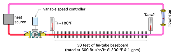
This circuit contains 50 feet of residential fin-tube baseboard, along with a variable speed circulator, flow meter, two temperature gauges and a heat source. That heat source is always controlled so the supply water temperature into the fin-tube element remains at 180F.

You turn on the circulator at full speed, and the flow meter indicates 8 gpm. The water temperature entering the fin-tube baseboard is steady at 180F, and after a short time the outlet temperature of the fin-tube element stabilizes at 174F.

Knowing the flow rate and temperature drop along the fin-tube, you can calculate the rate of heat dissipation.

Where:
q = rate of heat output (Btu/h)
D = density of the fluid (lb/ft3)
c = specific heat of fluid (Btu/lb/F)
f = flow rate (gpm)
∆T = delta-T, temperature drop (F)
8.01 = a number that makes the units correct

You now have a measurement of the heat output at a flow rate of 8 gpm. Next, you reduce the speed of the circulator so the flow rate drops by 1 gpm, wait for the outlet temperature from the fin-tube baseboard to stabilize, and write down the measured flow rate and outlet temperature.

You keep doing this for flow rates all the way down to 0.5 gpm, while the heat source always maintains the inlet temperature to the fin-tube baseboard at 180F.

Now that you’ve captured all this data, you can use it to calculate the temperature drop across the fin-tube element (e.g., delta-T), as well as the heat output rate from that element.

You then create graphs for heat output and temperature drop as a function of circuit flow rate.

They should look similar to the graphs in Figure 2 (below).

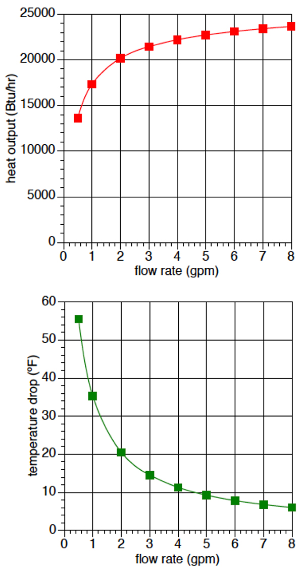
Figure 2. Heat output and temperature drop/flow rate.

It is what it is

The graph of heat output (q) versus flow rate is probably not what you expected—especially if you think proportionally. It shows that heat output from the fin-tube element drops off rather slowly as flow rate decreases, until you get down to a flow rate of about 2 gpm. Below 2 gpm the heat output drops quickly with any further reduction in flow rate.

Although it might not be what you expected, this non-proportional relationship between heat output and flow rate is reality.

This characteristic is shared by all hydronic heat emitters: fin-tube, convectors, panel radiators, and even radiant panel circuits.

Heat output changes very quickly at low flow rates, but very gradually at higher flow rates. This trend also holds true at other supply water temperatures.

Next, look at the temperature drop across the fin-tube over the same range of flow rates.

First, it’s obvious the temperature drop doesn’t remain constant as the flow rate changes. The ∆T happens to be at the commonly assumed value of 20F when the flow rate is just a bit over 2 gpm.

As flow increases above 2 gpm, the ∆T keeps dropping, and at 8 gpm it’s only about 6F.

When the flow is only 0.5 gpm the ∆T is slightly above 55F.

These ∆T values are the direct result of heat output. There’s nothing in this setup that forces the ∆T to stay at any particular value. There’s also nothing “wrong” with the fact that the ∆T is changing. It just goes where the physics takes it.

Another take away from this experiment is that there’s nothing special about operating a hydronic heating circuit with a temperature drop of 20F.

In Europe it’s common to see panel radiator circuits designed for design load ∆T of 30F or perhaps even higher.

European designers do this because it reduces flow rate, and reduced flow rate means small pipes and small circulators.

It also means lower operating cost. Over there, every watt counts. They won’t operate a circulator at 45 watts if it can create the necessary flow at 35 watts.

They care, and so should we, especially with increasing emphasis on mechanical systems for net zero buildings.

Radiant floor heating circuits can also be designed for different design load ∆T values. I like to design around 15F for floor circuits in areas that are expected to have “barefoot friendly” floors. The smaller ∆T reduces variation in floor surface temperature a bit compared to what it would be at a ∆T of 20F.

However, in an industrial building, I may push the design load ∆T for the circuit up to 25F. That’s because heated concrete slabs in most industrial buildings don’t need to be “barefoot friendly.”

Slightly wider variations in floor surface temperature are hard to notice through a pair of work boots. Designing around slightly larger circuit temperature drops also reduces flow rate, which in turn decrease circulator size requirements.

It’s not always intuitive

The relationship between the heat output of a hydronic circuit and the flow rate passing through it is not proportional.

Neither is the relationship between the circuit’s temperature drop and the flow rate through it.

Be sure to examine this relationship as you design future systems. Opportunities abound for reducing both installation and operating costs based on reduced flow rates and operating circuits at higher temperature drops. <>

John Siegenthaler, P.E., has over 40 years of experience designing modern hydronic heating systems and is the author of Modern Hydronic Heating (4th edition) and Heating with Renewable Energy (visit hydronicpros.com).